Convert sorted list to binary search tree

Leetcode link.

The way I handle this question is I first count how many nodes there are in the list, and construct an empty binary search tree, then use morris traversal/recursive inorder traversal to fill the whole tree with list value. Time complexity is O(n) with space complexity O(n).

But geekforgeek provided another brilliant solution. I am still pondering on why this works, and my bet is on the similarity between dfs and inorder traversal. But here is the code and some comments:

TreeNode* helper(ListNode* &head, int low, int high) {
    if(low == high) {
        TreeNode* ret = new TreeNode(head->val);
        head = head->next;
        return ret;
    }
    else if(low > high) return NULL;
    int mid = low + ((high-low)>>1);
    TreeNode* left = helper(head, low, mid-1);
    TreeNode* ret = new TreeNode(head->val);
    ret->left = left;
    head = head->next;
    ret->right = helper(head, mid+1, high);
    return ret;
}

TreeNode *sortedListToBST(ListNode *head) {
    if(!head) return NULL;
    ListNode* walker = head;
    int count = 0;
    while(walker) {
        ++count;
        walker = walker->next;
    }
    return helper(head, 0, count-1);
} 

That low and high index is quite confusing, they actually only represents how many nodes there are in this section. For each valid loop (\( low <= high \)) we need to make sure the list pointer moves to the next section once the root node for this section is handled, such that when we reaches line 13 list pointer is at the start of this section.
Anyway, this is the first time I see code that build a tree from leaf nodes. Very brilliant idea.

PS: geekforgeeks' code is actually even better than mine since the case when \(low == high\) is integrated in the ensuing code.

Divide Two Integers

Medium difficulty question with all kinds of corner cases, which bump the difficulty to hard.
Leetcode link.

Q: Divide two integers without using multiplication, division and mod operator.

A:
I managed to crack it by myself the first time I fought through leetcode, but not this time. I had to go back and check what I had done. :( shame

The idea is simple. Shifting operation is your friend. Test case \( \frac{700}{51} \): \[ 700 = 2^3 \cdot 51 + 292 \\ 292 = 2^2 \cdot 51 + 88 \\ 88 = 2^0 \cdot 51 + 37 \] We stop at 37 because \( 37 < 51 \).
All right that's it. Answer is \( 2^3+2^2+2^0 = 13 \).

Corner cases' time!

1. Dividend / Divisor == 0?
2. Dividient or Divisor is negative? or both are negative?
3. This is about integer, so what do you consider? Overflow! \(Dividend/divisor == INT\_MIN/INT\_MAX\) or \(-INT\_MIN/-INT\_MAX ?\)

First one is easy to handle. Notice when divisor is 0, throwing an exception is what you should do. But OJ says you can simply return 0. All right then.
Second one is tricky to handle. Judge the sign! Then use \( abs \) function to do it! Yeah, you'll see there is one loose end soon...
Third one? I cheated... I used long long type to handle everything. If I don't, the loose end in second question will reveal: The devil \( abs(INT\_MIN) \) !  ideone says \( abs(INT\_MIN) == INT\_MIN \), someone on leetcode forum reports \( abs(-2147483647) = -2147483644 \) or something like that. Anyway, I cheated...

My code is as follow. Not the best code though. Feel free to play it here.

pair<long long, long long> decompose(long long a, long long b) {        // DONT MAKE a < b
    int k = 0;                                  // decompose a/b = 2^k + d, d < 2^k
    while (b < a) {
        b <<= 1;
        k++;
    }
    if (b == a) return make_pair(k, 0);
    return make_pair(--k, a - (b>>1));
}

int divide(int dvd, int dvs) {
    if (dvs == 0) throw overflow_error("Divide by zero exception");
    if (dvd == 0) return 0;

    long long ldvd, ldvs;
    ldvd = abs((long long)dvd); ldvs = abs((long long)dvs);
    if (ldvd < ldvs) return 0;

    long long ret = 0;
    pair<long long, long long> kb;
    do{
        kb = decompose(ldvd, ldvs);
        ret += 1 << kb.first;
        ldvd = kb.second;
    } while (kb.second >= ldvs);
    return ((dvd>>31) == (dvs>>31)) ? ret : (~ret + 1);
}

Container with most water

Leetcode link:
Q:
Given n non-negative integers a₁, a₂, ..., a_n, where each represents a point at coordinate (i, a_i). n vertical lines are drawn such that the two endpoints of line i is at (i, a_i) and (i, 0). Find two lines, which together with x-axis forms a container, such that the container contains the most water.
Note: You may not slant the container. 


A:
Given line i and line j, one can easily come up with: \[ Area[i][j] = min(height[i], height[j]) * (j-i) \]
So an \( O(n^2) \) solution is fairly easy to get.


To decrease the time complexity, tricks and pruning are all what you need. Suppose we found an solution from i to j \( (i<j) \), and we assume \( height[i] < height[j] \). Then \( height[i] \) is dominant, which means if we decrease j, there will be no area larger than \( Area[i][j] \). This should be very easy to verify.


With this pruning, in order to investigate all possible i and j combinations, we start with \( i = 0 \) and \( j = height.size()-1 \) and shrink i and j inward, resulting the following simple code:

int maxArea(vector<int> &height) {
    if(height.size() <= 1) return 0;
    // idea of this program: If found one candidate [A[i], A[j]], 
    // if A[i] < A[j] then A[i] is dominate. all [A[i], A[j-k]] (k>0) 
    // will not generate area larger than [A[i], A[j]]. The only 
    // candidates can be achieved by moving j.
    int low, high;
    low = 0;
    high = height.size()-1;
    int maxarea = min(height[high], height[low]) * (high-low);
    while(low != high) {
        maxarea = max(maxarea, min(height[high], height[low]) * (high-low));
        if(height[low] < height[high]) low++;
        else high--;
    }
    return maxarea;
}

[Learning note]: Consistent hashing

This is a fun note. Original link here(Chinese), and here, here, here. (Update: it seems Amazon also use this stuff.)

So in the last post, I scratched the surface of amortized analysis. Amortize analysis shows that insertion in dynamic array is O(1) time complexity and so does insertion and deletion in hash map. But average analysis will have trouble in real world implementation. Consider the case below:

Problem statement

Map one object to \(N\) cache server can be done by a simple hash function \(hashkey(object)%N\). For uniformly distributed hashkey this algorithm is good.

Suppose we have 10 servers labeled as server 0 to server 9. Objects have hash key 11, 12 and 13. Then they will be mapped to server 1, server 2 and server 3.

What if:

1. One server (server 9) is down. Now the hash function changes to \(hashkey(object)%(N-1)\).
   
   In this case, objects have to be moved to server 2, server 3 and server 4. All objects have to be moved.
2. New server added. Now the hash function changes to \(hashkey(object)%(N+1)\).
   
   In this case, objects have to be moved to server 0, server 1 and server 2.

For large cache servers the cost of the above two cases are not tolerable. Consistent hashing is designed to minimize the compact of cache serve changes by minimizing key moves when new server is introduced or old server is removed from the system. Using our previous dynamic array example, when resizing or shrinking happens, consistent hashing is designed to minimize the resulting compact by reusing as many old keys as possible. As other posts, this post will mainly focus on the application side. More details can be found in this paper.

Algorithm Design

So as stated in Wikipedia and the reference link, circular hash space is used to represent a common modulo-based hash function. I will not redraw all the graphs this time, all figures credit to sparkliang.

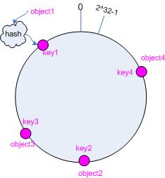
If unsigned 32-bit integer value is used as hash key, then the whole hash space can be referred to as a circular space based on modulo property. We represent it as the left figure below.

Given 4 objects with 4 different keys, the figure above shows their placement in the hash space. Up until here we are still using the classical hash design method.

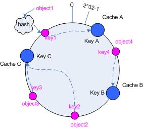
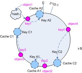
The innovative part of consistent hashing is, not only put object into hash space, cache server is also placed into the hash space. Suppose we have 3 servers. Using certain function, we map them two three different hash key Key A, Key B and Key C. Now place them to hash space:

Now we have object keys and server keys all in the hash space. The next question comes naturally: how to map objects to servers? You might have guessed it right already:

for each object we search clockwise (or counter-clockwise as long as you keep the direction consistent in your program design) and group it to the first cache server we find.

That's it. After grouping, the above figure is now:

Why is this consistent hashing method superior to the naive hashing method?

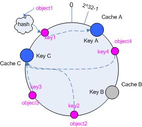
Let's revisit the two questions raised above and first discuss what happens when one server is down:

Suppose server B is down. Now based on the algorithm above, we have:

It is easy to see that only the segment between cache A and cache B needs to be processed. Comparing with the naive hashing method, removing a cache server causes relatively smaller impact.

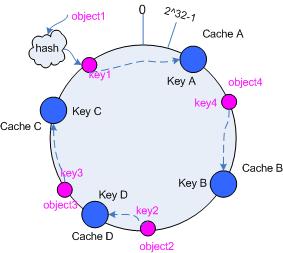
Adding a cache server is similar. Suppose a new cache server Cache D is added with Key D, we now have:

It is easy to see that only the segment between cache A and cache B needs to be processed, which brings better performance than naive hashing method.

Virtual cache server in hash space

Consider the following case (derived from cache deletion case):

In this case three objects are grouped to cache C while only one object is grouped to cache A. This balancing issue usually happens when we do not have too many cache server. To avoid this balancing issue, virtual servers are added to the hashing space such that we can mimic the behavior or many servers even though we have only a few servers.

The implementation is quite clever. For each server we make several replica. For example, for the case above, we make one shadow copy for each server and put the shadow copy back to the hashing space. Now we have:

And we can see the hashing space is balanced.

A simple simulation program has been written to verify that if different servers have different weight, for example a new server can take more work than an old server, replica number can be directly related to server weight. In the case of hash table resizing this technique is also applicable. Test link here.

[Learning note] Amortized analysis case: Dynamic array insertion complexity

Amortized analysis is sometimes used in algorithm analysis when average time complexity is more concerned than individual operations. I stumble upon this today when I am reviewing hash map implementation and find it fun.

Case 1: Dynamic array insertion

Consider a dynamic array of size N. When insertion is performed, if the dynamic array still has vacant locations, insertion will take O(1) time. But if the dynamic array is full (all almost full depends on the implementation), we will reallocate an array of size 2N and move original elements to this new array along with the newly added element. This single operation will cost about O(2N) time. (2N time to allocate the new array, at least constant time to delete the original array, N time to move the element, constant time to add the newly inserted element). So we will have a timeline similar to:

When amortized, resizing cost is distributed to all N insertions, leaving an average complexity of nearly O(1).

Case 2: Hash table resizing

With dynamic array insertion in mind, hash table resizing is quite similar. Consider a size N hashmap containing M elements. Its load factor is \( \frac{N}{M} \). The resizing scheme is as follow: If the load balance exceeds 1, we will double hash table size. If load balance is less than \( \frac{1}{4} \), hash table size is halve.

Use the same analyzing scheme, the amortized cost for insertion is calculated as: (Figure redrawn from here.)

When amortized, the average cost is still O(1).

As to shrinking hash table, we start with \( N = \frac{M}{2} \) since this is what remains after one last shrinking operation. We need to perform at least \( \frac{M}{4} \) deletion operations before another shrinking is needed. This shrinking will have time cost of O( \( \frac{M}{2}\) ). Distribute this time to all \( \frac{M}{4} \) deletion operations. The amortized time complexity is still O(1).